Implementing the count-min sketch in Owl

This post describes my project implementing the count-min sketch in OCaml as part of the Owl library for scientific computing. This work was conducted under the supervision of Professor KC Sivaramakrishnan, with guidance from Professor Yadu Vasudev, at the Indian Institute of Technology Madras during summer 2019.

The count-min sketch

The count-min sketch is a probabilistic data structure that provides an approximate frequency table over some stream of data. At the cost of returning possibly inaccurate results, the sketch requires memory usage and query times that are independent of the contained data. Variants of this sketch have been proposed for a variety of networking applications and in MapReduce/Hadoop implementations, and existing implementations include Twitter’s algebird library. The data structure supports the following two operations:

• incr(v): increment the count of value v
• count(v): get the current frequency count of value v

The count-min sketch consists of essentially the same structure as a Bloom filter. It maintains a two-dimensional table t of counters, containing l rows each of length w. Associated with row j is a hash function \(h_j : U \mapsto \{0,1,\dots,w-1\}\), where \(U\) is the set of all possible input values. Each counter is initialized to 0. incr(v) increments the values at t[j][h_j(v)] for j in {0,1,...,l-1}. Thus, the data structure maintains l separate counts of each element put in. However, due to hash collisions these counters may differ from the true count. Note that the error in each counter can only be positive, since counters are only ever increased rather than decreased. Thus, the best estimator for the true count of an element is the minimum of all the corresponding counter values. So count(v) returns min(t[j][h_j(v)] over j in {0,1,...,w-1}).

The count-min sketch is typically parameterized in terms of \(\epsilon\), the approximation ratio, and \(\delta\), the failure probability. Given these parameters, the sketch provides the following guarantee:

For all values v in input stream S, letting f(v) be the true frequency of v in S:

• count(v) \(\geq\) f(v)
• with probability at least \(1 - \delta\):
  • count(v) \(-\) f(v) \(< \epsilon \times ||S||_1\)

where \(||S||_1\) is the \(L_1\) norm of S, equal to the total number of elements in S.

It can be shown that this guarantee is achieved by setting \(w = \Theta(\frac{1}{\epsilon})\) and \(l = \Theta(\log(\frac{1}{\delta}))\). Thus, the memory size of the sketch is \(\Theta(\frac{1}{\epsilon} \log(\frac{1}{\delta}))\), and the time to execute count and incr are \(\Theta(\log(\frac{1}{\delta}))\). (See proof here or here).

Note that these resource usages are independent of both \(||S||_1\) and the number of distinct elements of S. Contrast this to the most common implementation of a frequency table–using a hash table to store (value, count) pairs. The size of the hash table scales as the number of distinct values encountered in the stream, which is \(O(||S||_1)\).

The cost of this very low resource usage is some inaccuracy in the estimated frequencies. Note that the error is bounded by \(||S||_1\), meaning that the sketch can give very inaccurate results for highly infrequent elements, but is guaranteed (with high probability) to give good estimates for the most frequent elements. Thus, the sketch is most useful for problems in which we are concerned with the most common elements in the stream.

The heavy-hitters sketch

The simplest problem for which a count-min sketch is used is simply finding the frequent elements in a stream: the \(k\)-heavy hitters problem. The \(k\)-heavy hitters in a data set are those elements whose relative frequency is greater than \(1/k\). We can use the count-min sketch to build a heavy-hitters sketch, which supports the following operations:

• add(v): increment the count of value v
• get(): return the k-heavy hitters and their frequencies

The heavy hitters sketch is parameterized in terms of \(k\), \(\epsilon\), and \(\delta\). It provides the following guarantee:
With probability at least \(1 - \delta\), the data structure

• outputs every element that appears at least \(\frac n k\) times, and
• outputs only elements which appear at least \(\frac{n}{k} - \epsilon n\) times.
  Note that for the sketch to give useful results, we should set \(\epsilon < 1/k\).

Note that the count-min sketch does not actually store the values whose frequencies it counts, instead relying on hashing to make the counts retrievable. Indeed, simply storing each value would get us to the same asymptotic memory usage as a hash table, thus defeating the point of the sketch. But in the heavy hitters case, we need to maintain the actual values of the heavy hitters as well as their frequencies. This is done using a min-heap. In addition to a count-min sketch for frequencies, the heavy hitters sketch maintains a min-heap of the elements currently considered to be heavy hitters. Whenever add(v) is called, first incr(v) is called on the underlying count-min sketch. Then, count(v) is called to get the current count of v. If this count is greater than \(n/k\) (where \(n\) is the total number of elements added so far), then the pair (v, count(v)) is added to the min-heap. If a pair containing v is already present in the heap, then its position is adjusted to reflect the new count. Finally, we remove elements whose frequency is too low to be a heavy hitter: while the minimum element in the heap has frequency less than \(n/k\), we remove the minimum element. To implement get(), we simply transform the heap into a list or array and return it.

The memory usage is that used by the count-min sketch and the min-heap. Note that the maximum size of the heap is the number of heavy-hitters, which is \(O(k)\). Thus, the total memory usage is \(\Theta(\frac{1}{\epsilon} \log(\frac{1}{\delta}) + k)\). The update time is \(\Theta(\log(\frac{1}{\delta}) + k)\).

Implementation

My implementation was designed so as to be as minimal as possible, allowing the user to choose how data is input. Additionally, I wanted to make it easy to use the sketches in an “online” situation, where data arrive continuously and frequency information can be requested at any time. There were a few issues that I came across when designing and implementing the sketch.

Different types of table

The count-min sketch requires an underlying table to store the counters, and there were a couple of choices for this. OCaml provides a native array data structure, while Owl provides various types of ndarray built on top of the OCaml Bigarray. The Owl ndarray is designed to support complex operations like slicing very efficiently, but the sketch only requires getting and setting a handful of individual values in each operation. Since the sketch is independent of the underlying implementation of the table, I decided to functorize my implementation to abstract this out. I first wrote a signature Owl_countmin_table.Sig which defines a type t for tables and initialization, increment, and get functions over it. I then wrote two implementations, Owl_countmin_table.Native and Owl_countmin_table.Owl, using the OCaml array and the Owl ndarray respectively. Owl ndarrays are available only with floating-point or complex values, so I chose a single-precision floating point value since we never use the decimal part. Finally, the actual count-min sketch was implemented as the functor Owl.Countmin_sketch.Make, which takes a module with signature Owl_countmin_table.Sig.

As explained later, this proved unnecessary since the native array outperformed the Owl array in all respects. However, I still feel it was a useful exercise since it ultimately made the code for the sketch more readable.

Hashing

The count-min sketch requires a pairwise independent hash function family, from which the \(h_j\) are drawn. The simplest family of such hash functions is just \(h(x) = (ax + b) \mod p\), where \(p\) is a prime and \(a, b\) are drawn uniformly at random from \(\{0,1,\dots,p-1\}\). A good choice for \(p\) is \(2147483647 = 2^{31} - 1\). In binary, this \(p\) is 30 1s, so taking \(x \mod p\) can be accomplished by applying a bitwise AND to \(x\) and \(p\). Finally, we need to take \(\mod w\) to get an index into the length-\(w\) row of the count-min table.

To make the sketches polymorphic, we need a hash function that can take any value and return an integer. This is not trivial in OCaml, but fortunately the Hashtbl module provides Hashtbl.hash which does exactly this. So incr s x first takes Hashtbl.hash x, then applies the above \((ax + b) \mod p\) function.

Heavy-hitters heap implementation

One issue I ran into during development was how to implement a min-heap priority queue for the heavy-hitters sketch. The OCaml standard library doesn’t have one built in, and it’s not natural to write an array-based heap in a functional language like OCaml. Fortunately, Owl did have a heap implementation already built. However, this implementation (along with most existing implementations) doesn’t support the decreaseKey operation, which adjusts the priority of an element already in the heap and is commonly assumed in theoretical work. I spent some time attempting to modify the Owl implementation, but this turned out not to be effective. decreaseKey requires the data structure to remember the location of each element in the heap, and building this additional structure added a lot of bloat and complexity to the code. Instead, I ultimately decided to use OCaml’s native Set data structure, which is implemented using balanced binary trees and thus has a notion of ordering. While this made the code a lot more readable, it does mean that the runtime of add is linear in the number of heavy hitters. I decided this was an acceptable tradeoff since the number of heavy hitters is O(k), and the heavy-hitters sketch already has a time dependency on k.

However, using the OCaml native set presented its own problems. The native set is provided as a functor which requires a module containing the type to be stored and a comparison function over those types. However, the type of elements to be stored is 'a * int, meaning that we cannot directly use the Set.Make functor with a fixed type in our implementation. Instead, I used first-class modules to package up the output of the Set.Make functor within the heavy-hitters data structure. I’d never used this technique before, but it ended up being quite elegant.

Benchmarking and testing

Once the implementation was done, I had to test it. At first I just used simple tests based on generating random integers from various statistical distributions, but something more robust than this was required. The major difficulty with testing an approximate, probabilistic data structure like this sketch is that the expected output is only approximately known—the sketch can return frequencies that differ from the true frequencies in the underlying data without there necessarily being an error in the implementation. For this reason, I had to use average measures of error when testing.

I also benchmarked my implementation to understand the performance boost it gives over the naive hash-table solution, and to determine which of the two tables was more efficient.

Comparing the two table implementations

To test the two tables, I wrote a simple script that inserted n elements drawn from a provided distribution into a sketch with parameters epsilon and delta, then queried the sketch for the counts of n more elements drawn from the same distribution. I recorded the time for each incr and get operation using Unix.gettimeofday, being sure to call Gc.compact before calling the operation such that time spent in the garbage collector did not affect my measurements. I found that the OCaml native array implementation was about 40% faster (0.23s vs 0.33s for \(10^5\) operations) on incr and 10% faster (0.30s vs 0.33s for \(10^5\) operations) on count compared to the Owl ndarray implementation.

For memory, I used the live_words statistic provided by the Gc module, which measures the total number of words maintained in the OCaml heap. I measured the heap size before the structure was allocated and throughout the sequence of incr and count operations. However, I found that using this metric, the Owl ndarray implementation appeared in some cases to use zero memory! This is because the Owl ndarray is built on top of the OCaml Bigarray, which is designed to allow cross-operation with C and Fortran arrays. The Bigarray array is actually allocated via an FFI to C code, and thus is not included in the OCaml GC heap. So just using live_words from the OCaml Gc was not actually measuring the size of these arrays.

To rectify this, I wrote a small utility called ocaml-getrusage which is a thin OCaml wrapper for the getrusage Unix system call. getrusage returns a struct containing various different statistics pertaining to the resource usage of a process. I used the OCaml C FFI to write a thin wrapper around the function. With this tool, I found that the Owl ndarray generally used about 10-20% more memory than the native array for the same parameters epsilon and delta.

Since the native array outperforms the Owl ndarray in both speed and memory usage, the native implementation (Owl_base.Countmin_sketch.Native) should be preferred.

Comparing to the naive implementation

I also wanted to measure the performance of the sketch against a naive hash-table-based frequency table, which I wrote using the OCaml Hashtbl module. I used the news.txt corpus available here, comprising online news articles containing a total of about 61 million words. I wrote a script that ran both a count-min sketch and a hash-table over this dataset, then extracted the frequencies of each unique word in both data structures and compared them. I also measured the total memory usage for both structures in the same way as described above. (Since I only measured using the native implementation, using Gc heap words was valid.) The first problem I ran into with this approach was that the average relative error rate was enormous, often on the order of about 100,000%. This was due to large errors in the estimated count-min frequency of very uncommon words. Since most words appear very infrequently, this leads to a large average error rate when the average is taken over all unique words. Instead, bearing in mind that the typical use case of the sketch is to get information about frequent elements in the data, I decided to take the average over only elements with a relative frequency greater than phi. Using this approach, I generated the following plot showing the tradeoff between memory usage and accuracy:

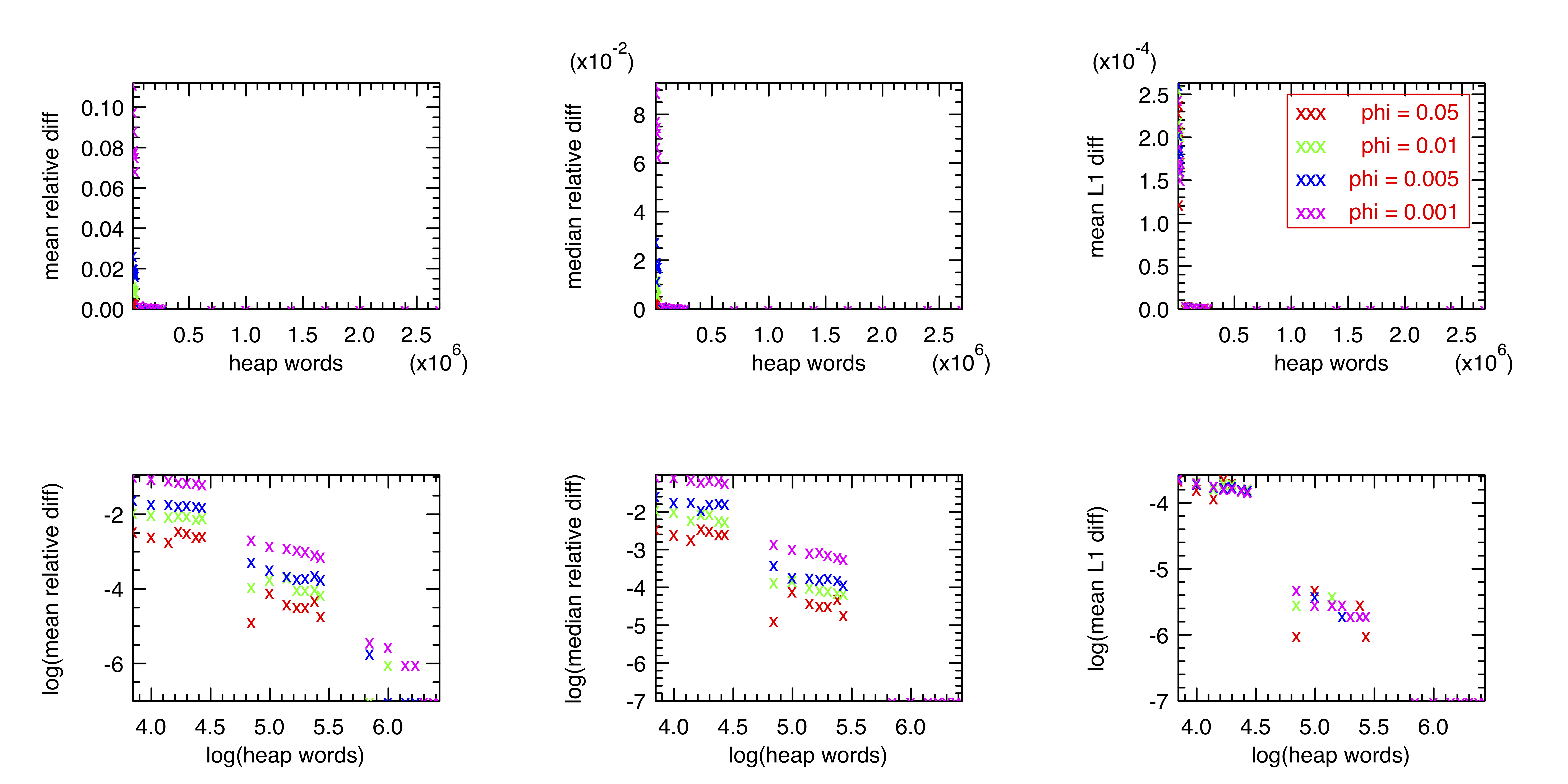
The three measures of error are the mean relative difference in frequency, median relative difference in frequency, and mean difference in frequency relative to the L1 norm of the whole dataset. The ranges used were: epsilon in [0.00001, 0.01], delta in [0.0001, 0.01], phi in [0.001, 0.05]. On my 64-bit machine, one heap word is 8 bytes, meaning that the sketches ranged in size from 5.6 KB to 11.2 MB. Compare this to the hash-table implementation, which used about 25 MB. As expected, larger tables resulted in a lower error rate. There appeared to be an approximate power law relationship, meaning that small changes to epsilon and delta could lead to very large changes in the accuracy of the sketch; my own experience testing and debugging my implementation matches this. Combined with the difficulty of defining and measuring accuracy, this means that users of the sketch must experiment with these parameters to determine an appropriate balance for their particular situation. However, there are clear benefits to using the sketch versus a simple hash table in cases where absolute precision is not required and only the most frequent elements are of interest.

Ongoing and future work

This implementation already provides the basic functionality of the sketch, which is sufficient for a number of the previously mentioned applications. However, some avenues for further work exist. For me, one of the most interesting of these is to allow for distribution of the sketch over several separate processors or devices. Note that if two sketches are initialized with the exact same hash functions and table size, they can be combined at any time by simply adding the two tables element-by-element. We could imagine a situation where many small, resource-constrained devices are running in a distributed network, but we still want to be able to query the whole network for overall frequency information. In this case, initializing a sketch with the same hash functions on each device would allow us to maintain the frequency table such a way. I have begun to implement and test this functionality on top of my implementation.

Acknowledgements

This work was funded by a Harvard OCS undergraduate travel and research grant. I am very grateful to Liang Wang, Richard Mortier, and others at OCaml Labs for their guidance on aspects of this project.